Lab 2. Tree Building with UPGMA
February 13 & 14, 2024
02_biol_200_lab_2.RmdNotes:
Read this entire handout and complete the Prelab Exercise, submitting it BEFORE you come to lab.
Turn in your assignment via the link on the lab website: https://gledits2.github.io/biol_200/index.html
Please bring Lab 1, including your completed tree. Please bring a calculator.
Make sure you are familiar with new terms before coming to lab. We suggest you build your own personal vocabulary notebook by writing out definitions. Use the glossary or index of your text, lecture notes, an online dictionary, etc. There are also excellent biological dictionaries in the reference section of the Science Library.
Objectives:
Understand characters and character states as applied to phylogenetics.
Use the scientific process as an investigative tool.
Visit the greenhouse and practice scoring character states on live plants.
Learn the UPGMA algorithm for building a tree from your own data.
KEY WORDS: character; character state; systematics; morphology; ancestral; derived; UPGMA; algorithm; dendrogram; cladogram
1 Overview
Last week we learned how to read and interpret phylogenetic trees. But how do we know how species are related phylogenetically? At some level, we all have an intuitive sense of some species relationships. For example, it’s probably fair to say that everyone knows that lions are more closely related to jaguars than they are to wolves, right? Lions just look much more like jaguars than they do wolves. But let’s think of a more specific example: are lions more closely related to tigers or to jaguars? That’s not so intuitive, is it?How could we infer the phylogeny of these organisms?
Accurately reconstructing evolutionary relationships requires comparing characteristics of organisms in a rigorous, empirical framework. (Incidentally, the accurate reconstruction of phylogenetic relationships is one of the core goals of systematics, which is the field of biology that is concerned with understanding the diversity and phylogenetic interrelationships of life.) What characteristics of an organism can we use to determine phylogeny? There are lots of possibilities, but perhaps the first thing that comes to mind is the use of morphology (or anatomical traits). For example, we might try to think of all the morphological traits that unite lions and jaguars, or lions and tigers, etc. You could probably also think of non-morphological traits that might be useful in assessing relationships—cellular and molecular traits like chromosome number, protein similarity, and even DNA sequence. What about a type of behavior? Could that be a character?
When comparing traits among organisms in a phylogenetic context, it is important to understand the terms character and character state. Essentially, a character is a trait, and a character state is the particular version of that trait which happens to be present in a given taxon. For example, different species of flowering plants all have flowers, but they may have differing numbers of petals. Some species may have five petals, some may have three, and some may have none at all (for example, wind-pollinated plants). In this example, the character is “number of petals” and the character states are “5”, “3”, and “0”. There are numerous ways to infer phylogeny, but all of the various methods share one thing in common: they all explicitly utilize characters and character states.
One of the main purposes of this week’s lab is to give you some real-world experience with characters and character states. First, in the pre-lab exercise you will practice defining characters and character states in the fictitious plant genus Oberlinia. Then, during the lab period, we will take you up to the greenhouse to practice “scoring” (i.e. assigning) character states on real plants. Finally, you will use your scores of morphological character states from the greenhouse plants to infer the phylogeny of these taxa.
This lab also provides an excellent opportunity to think about the scientific process. Remember that the goal of science is nothing more than answering questions. Today we ask, “What are the relationships among a set of taxa?” As you work through the exercises in this lab, be thinking about, and ready to discuss, how the stages of the scientific process apply to phylogenetics. What are we observing? What are our hypotheses? How do we test our hypotheses? How is it repeatable?
2 Characters and character states in Oberlinia
Find the Oberlinia Specimen Sheet and the character state matrix (the Oberlinia specimens can also be found below). On the specimen sheet are the fictitious Oberlinia “taxa” (labeled A–I) we will use to practice characters and character states. Take a look at them and think about how the different species seem to differ from one another. Can you think of some characters and the character states that are present among these 9 species of Oberlinia? On the character state matrix, taxa are listed on the left and spaces for 5 characters are given on the top. We have given you an example of one possible character that could be defined and scored for all nine species. Using this example as a guide, refer to the Pre-lab Exercise and answer Question 1 by defining/listing five additional characters that could be scored for Oberlinia, and then score the character states using the blank matrix. Think about the characters you chose; might some character state designations be more empirical or repeatable than others? For example, if you chose ‘petal size’ as a character, and ‘large’ or ‘small’ as character states, consider different criteria you might have used.
Oberlinia Specimens
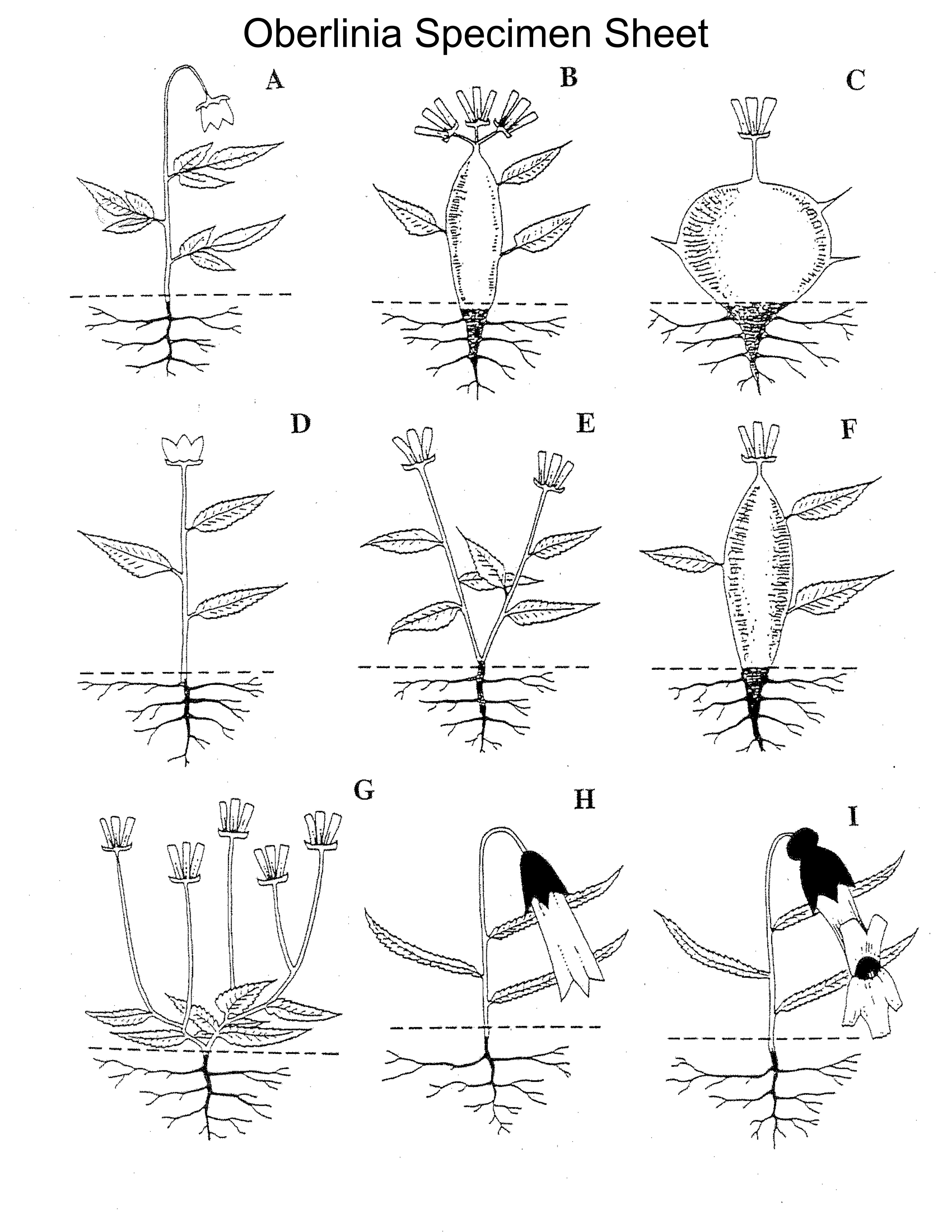
Consider this other important topic related to character states—determining which are ancestral (those traits that were present in the last common ancestor of a clade) and which are derived (those traits that newly appear within some lineage). For a particular clade, there can only be one ancestral character state for each character, but there can be many derived character states. Keep in mind that ancestral and derived are relative terms; in other words, they always apply to a specific clade. Here’s an example of the relative nature of the terms: when viewing the clade Mammalia (mammals) alone, the presence of mammary glands is the ancestral character state for the clade; however, if we look at the clade of all vertebrates (which includes mammals), then presence of mammary glands is certainly not the ancestral state—instead, in this context, it is a derived state.
Take a look at your character state matrix for Oberlinia. Answer Question 2 of the Pre-lab Exercise: Given the character states you came up with, try to determine which character state was ancestral for Oberlinia for a few of your characters. This task may be somewhat difficult in some characters, and you may realize that you made preconceived judgments about which characters were ancestral and which were derived in order to draw your tree. Does this seem very “scientific”? How would you avoid such scientific missteps?
We will return to the notion of ancestral and derived character states another time. For now, you can practice this concept on your own by determining ancestral and derived character states for various characters in the phylogeny on the Tree of Life Sheet from Lab 1 – complete Question 3-7 of the Pre-lab Exercise. (Keep in mind that the character states on this handout are mainly presence/absence character states. For example, were mammary glands present or absent?)
3 Scoring character states for DNA
Below is a fictitious DNA matrix for 11 species of Oberlinia. Each row contains a different 20-base nucleotide sequence that can be read left to right; the numbers at the top indicate the nucleotide position, from 1-20. Let’s think about how we might treat these sequences as characters and character states.
Consider the DNA matrix above and our earlier discussions of character. Answer questions 8-10 of the Pre-lab Exercise:
- What do you think we would treat as a character in this matrix?
- What are the possible character states for each character?
- Which of these sources of characters do you think is
“best”—morphology or DNA sequence? In other words, which do you think
will give a more accurate view of phylogeny? Try to make a prediction
now and try to justify your decision.
4 During lab: Discussion of characters/character states in Oberlinia
During lab, in your groups, discuss your Oberlinia character matrix (don’t forget to also look at the taxa!). Take five minutes to have a discussion with your group members about the characters you chose, and whether some character state designations might be more empirical or repeatable than others.
How would we determine relationships between these species? Take a minute to look over all the species. Then, decide among yourselves what you think the evolutionary relationships between these nine species are. Draw a phylogenetic tree depicting these relationships.
After you’ve finished drawing your tree, discuss the following questions within your group: What char-acters and character states did you rely on to make your decisions about relationships when drawing the tree? Do you think that was a satisfactory way of elucidating phylogeny? In other words, should we make educated guesses?
How would we make this process more explicit? There are many possibilities, but all of them rely on defining characters to be scored and then scoring the character states for each species.
5 Scoring character states in the greenhouse
Now let’s do a real-world example of character state scoring. Today you will begin a project to reconstruct the phylogenetic relationships between 10 plant species growing in Oberlin’s greenhouse. We will use data sets of morphology (today) and DNA sequence (in a few weeks) to compare the phylogenies that we obtain. Your lab instructor or TA will take you up to the greenhouse to score morphological character states for these 10 species. To ensure that each lab group can compare their results, we have selected the 6 characters for you and have provided you with a set of character states that can be scored for each character (handout available during lab). This exercise is also a great way for you to learn a little more about plant morphology.
DNA has also been extracted from the leaves of these species and sequenced for the rbcL gene. In a few weeks, we will return to this group of taxa to consider the phylogeny inferred from the DNA characters and compare with the tree inferred from morphological characters.
Doing this phylogenetic exercise will give you a sense of what systematics is all about and will lay a strong foundation for understanding other aspects of biodiversity and evolution that will be covered in this course. Plus, this exercise will help reinforce the notion that an accurate phylogeny is absolutely necessary for any type of comparative biology.
6 Introduction to tree building with UPGMA
How do we convert the data in these character state matrices into a
phylogeny? There are many ways to infer phylogeny, but all utilize
characters and character states. In the greenhouse, you scored
morphological character states to create a character state
matrix; now you will learn a simple technique,
UPGMA, to convert these data into values of
The UPGMA
(
Below is an example of a tree generated by UPGMA. The first thing to
keep in mind when reading this tree is that it depicts
Take a look at taxa A and B in the tree (below). The length of the horizontal branches that separate A and B (there are two branches!) is equal to 0.3 (each branch is 0.15 in length). To determine the index of similarity for this pair of taxa, you simply subtract this number from 1, which yields 1 - 0.3 = 0.7. This index indicates that these taxa share 70% of their character states. In other words, adding up the branches that separate two taxa yields the amount of difference between them (index of dissimilarity); you need to subtract this number from 1 to get the index of similarity. As you work through this algorithm, make sure to keep in mind which index you are using for which processes.
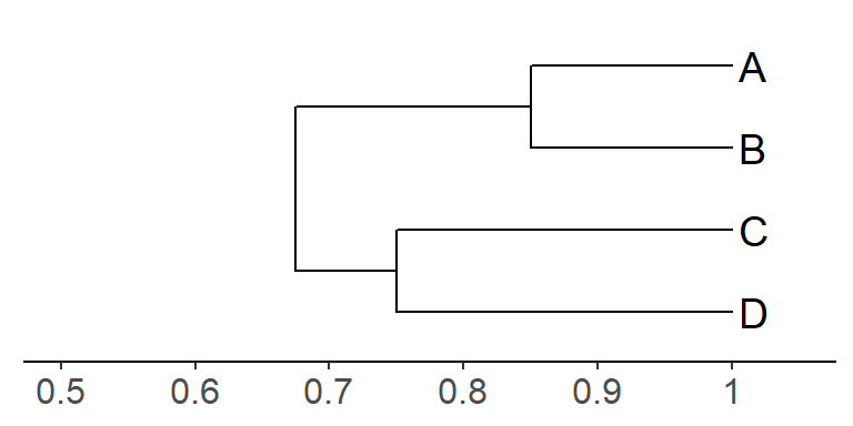
In the example above, the index of similarity between taxa A and D is 0.34. Can you determine how that number was derived, using the information in the above tree? Figure this out with your group.
The UPGMA algorithm is described below, with an example.
6.A UPGMA Algorithm, with and Example
The best way to learn is by doing. With your partner, use the following example as a guide to create your own similarity matrices and UPGMA tree using six of the greenhouse species you looked at today.
Step 1: Convert the original character matrix to a similarity matrix.
In the example character state matrix below, there are 5 taxa and 4
characters. The first thing we want to do is to calculate the similarity
between
Taxon |
No. of Petals |
Flower Color |
Leaf Margin |
Fruit Type |
|---|---|---|---|---|
A |
4 |
Yellow |
Entire |
Drupe |
B |
8 |
Yellow |
Serrate |
Berry |
C |
8 |
Orange |
Serrate |
Berry |
D |
8 |
Yellow |
Serrate |
Drupe |
E |
8 |
Orange |
Serrate |
Berry |
To calculate the similarity matrix, calculate the following value for each pair of taxa:
\[Similarity ~ of ~ taxa ~ X ~ and ~ Y = S_{XY} = \left(\frac{Number ~ of ~ shared ~ character ~ states}{Total ~ number ~ of ~ characters}\right)\]
Report your calculations to three decimal places. Here’s the finished similarity matrix:
Taxon |
A |
B |
C |
D |
E |
|---|---|---|---|---|---|
A |
|
0.25 |
0 |
0.5 |
0 |
B |
|
|
0.75 |
0.75 |
0.75 |
C |
|
|
|
0.5 |
1 |
D |
|
|
|
|
0.5 |
E |
|
|
|
|
|
(Think: Why don’t we have to fill out the other side of the matrix?)
Step 2: Find the taxa with the highest similarity value and join them together.
The length of each horizontal branch that connects a pair of taxa should be equal to half the distance between them (e.g., if two taxa have a similarity value of 0.75—in other words, a distance of 0.25—then each branch would be 0.125 units in length).
In this case, C and E have the highest similarity (1.0—i.e. they share 100% of all character states), so we join them together to start a tree (notice the scale bar at the bottom!):
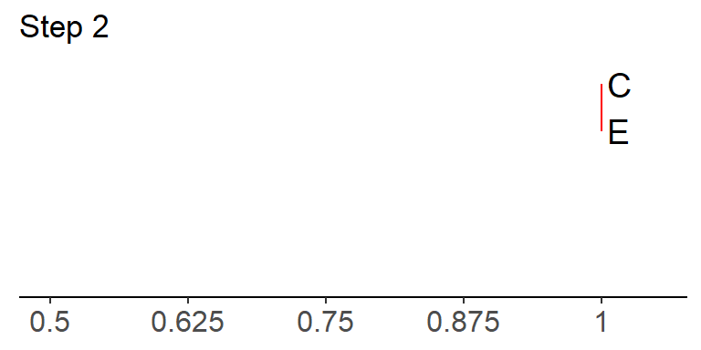
In the above example, there is no horizontal branch length between C and E because there is no difference between them—remember that horizontal branches indicate dissimilarity in UPGMA.
Step 3: Recalculate the similarity matrix, treating C and E as a unit.
To determine the similarity values for the composite taxon C/E, take the average of the similarity values of C to a given taxon and E to a given taxon, using the similarity values in the ORIGINAL similarity matrix above.
For example, the similarity of:
\[C/E ~ to ~ A = \frac{\left(S_{CA} + S_{EA}\right)}{2} = \frac{\left(0 + 0\right)}{2} = 0\]
\[C/E ~ to ~ B = \frac{\left(S_{CB} + S_{EB}\right)}{2} = \frac{\left(0.75 + 0.75\right)}{2} = 0.75\]
\[C/E ~ to ~ D = \frac{\left(S_{CD} + S_{ED}\right)}{2} = \frac{\left(0.5 + 0.5\right)}{2} = 0.5\]
Here’s what the new matrix would look like:
Taxon |
A |
B |
C/E |
D |
|---|---|---|---|---|
A |
|
0.25 |
0 |
0.5 |
B |
|
|
0.75 |
0.75 |
C/E |
|
|
|
0.5 |
D |
|
|
|
|
Step 4: Join the two values with the highest similarity value in the matrix in step 3, using the appropriate branch lengths.
There is a tie! The similarity value of B to C/E and that of B to D are both 0.75. Because taxon B is present in both comparisons in this example, there will be two alternate trees that can be calculated, both of which are equally valid. In these cases, you can choose to proceed with any of the highest values. We will continue below with the tree that joins B to C/E.
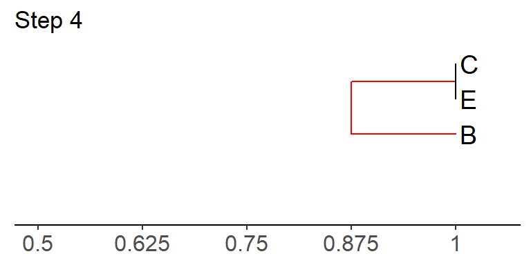
How were the branch lengths calculated above? To do this, first find
the similarity value for B and C/E in the above matrix (0.75). This
means that B and C/E are 25% dissimilar (1 - 0.75 = 0.25),
which means that the total branch length between B and C/E
should be 0.25. We divide this length in half; i.e. 0.25/2 = 0.125. So
this means that the branch from taxon B to the node uniting B, C, and E
should equal 0.125 (look in the tree above), as should the branch
leading from this node to BOTH taxon C and E. In other words, the total
branch length from B to C
(
Step 5: Recalculate the similarity matrix, treating B, C, and E as a unit.
To calculate similarity values for the composite taxon B/C/E (again,
refer back to the
The similarity of:
\[B/C/E ~ to ~ A = \frac{\left(S_{BA} + S_{CA} + S_{EA}\right)}{3} = \frac{\left(0.25 + 0 + 0\right)}{3} = 0.08\]
\[B/C/E ~ to ~ D = \frac{\left(S_{BD} + S_{CD} + S_{ED}\right)}{3} = \frac{\left(0.75 + 0.5 + 0.5\right)}{3} = 0.58\]
Taxon |
A |
B/C/E |
C |
|---|---|---|---|
A |
|
0.08 |
0 |
B/C/E |
|
|
0.58 |
D |
|
|
|
Step 6: Join the two values with the highest similarity value in the matrix in step 5, using the appropriate branch lengths.
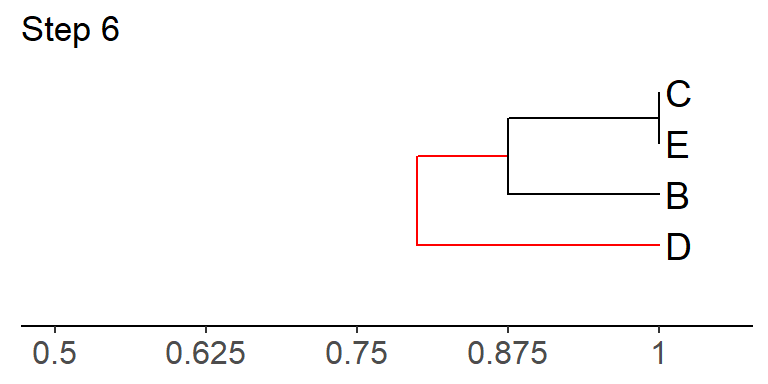
How was the branch length leading to D calculated? Can you duplicate this?
Step 7: Calculate the similarity between A and the composite taxon B/D/C/E, and add A to the tree using the appropriate branch lengths.
The similarity of:
\[B/C/D/E ~ to ~ A = \frac{\left(S_{BA} + S_{CA} + S_{DA} + S_{EA}\right)}{4} = \frac{\left(0.25 + 0 + 0.5 + 0\right)}{4} = 0.19\]
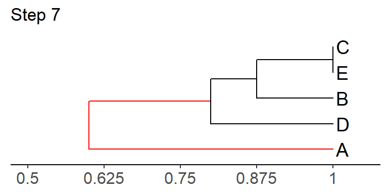
And that’s it! We’re done!
Now, go ahead and practice building a UPGMA tree for 6 of the 10
greenhouse taxa.
7 Post-Lab Assignment – due at start of Lab 3.
Turn in your completed:
- UPGMA similarity matrices (handed out in lab)
- Labeled UPGMA tree (make sure you include the scale and have indicated the numerical position where each vertical line would intersect the x-axis).
Please be sure to
8 Pre-lab Exercise
Turn in before start of lab period.
You should have read the lab write-up before attempting this exercise.
Questions:
- Fill in the table below with the characters and character states that you described:
Character |
Possible character states |
|---|---|
Leaf Width |
Broad, Absent, Narrow |
_ |
_ |
_ |
_ |
_ |
_ |
_ |
_ |
_ |
_ |
- After defining characters for the Oberlinia taxa, can you determine which character states are ancestral for some of your Oberlinia characters?
Examine your Tree of Life sheet from Lab 1 for the following questions.
- Which character state is a unique derived character state for angiosperms?
- List one character state that is ancestral to the clade of angiosperms and gymnosperms.
- What character state on the tree is derived for Class Aves but not Class Mammalia?
- Find an example yourself. Choose two terminal taxa and determine what the derived/ancestral state is for a character.
- For the clade that includes the two terminal taxa you chose, determine a shared derived character state that is unique to that clade.
Refer to section 3 Scoring character states for DNA for these questions.
- What do you think we would treat as a character in the Oberlinia DNA matrix in Section 3?
- What are the possible character states for each character in the DNA matrix?
- Which of these sources of characters do you think is “best”—morphology or DNA sequence? In other words, which do you think will give a more accurate view of phylogeny? Try to make a prediction now and try to justify your decision.